When is a bigger model actually better? A practical framework for model routing

Model routing is an increasingly common way to give users more value by balancing speed, accuracy and cost systematically. One setup is to have two (or more) models that solve the same task, one which is optimized for speed and cost vs. one which is slower and more capable.

We explored this setup on one internal task at Reducto, where our datasets showed that some types of pages parsed fine with a faster model while others benefited significantly from a more capable one. That variation made it a useful setting for studying routing and the tradeoff between quality and latency.

Formalizing the router

Suppose we have a set of requests and for each request i, we must choose one of two models. Let δᵢ = score(big) − score(small) be the quality gain from escalating request i to the larger model, and let cᵢ be the resource cost that escalation causes (e.g. incremental compute cost, or added latency). A routing policy is then a binary vector x, where xᵢ = 1 means we escalate.

What should the policy maximize? Quality, obviously, but not unconditionally. If quality were free we would escalate everything. We instead maximize a constrained objective which additionally considers cᵢ:

maximize Σ xᵢδᵢ, subject to Σ xᵢcᵢ ≤ B

for some budget B. In production, B is best read as a long-run average resource budget (e.g. added latency per request, GPU-seconds per minute, dollars per thousand requests). If we introduce a multiplier λ on the budget constraint and consider its Lagrangian relaxation, the routing decision decomposes across requests: escalate i exactly when

δᵢ − λcᵢ > 0

This formulation reveals two notable findings:

1. The magnitude of δᵢ matters, and the point at which escalation stops paying for itself is set by λ.
2. λ carries the entire budget. It is a serving-time scalar, so one pair of predictors supports every budget the product might want, and each budget is just a different point on one curve. You can hand λ to the user, or set it per workload, without retraining anything.

If cᵢ is roughly constant across requests, δᵢ − λcᵢ collapses to ranking by δᵢ and routing becomes an ordering problem. If costs vary, the ordering induced by δᵢ − λcᵢ moves with λ.

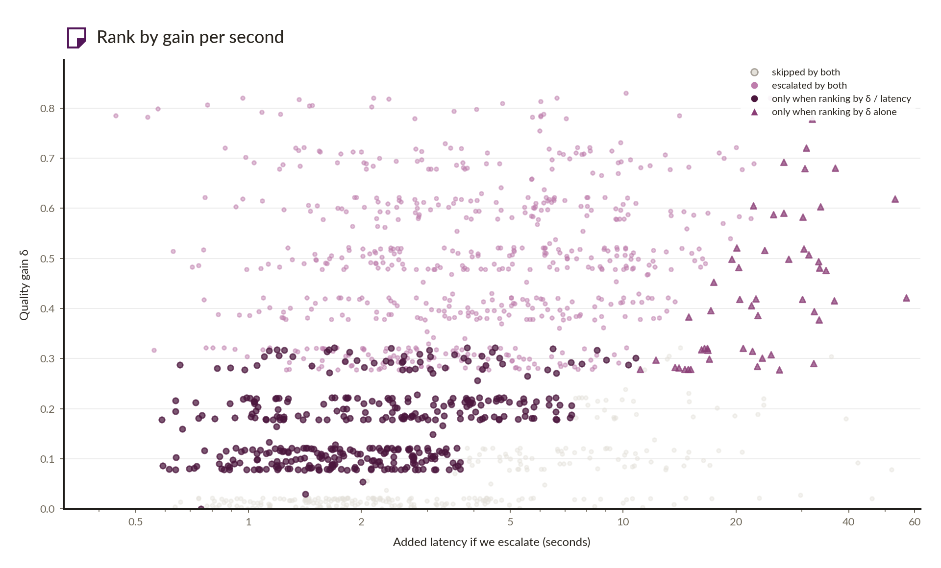
The difficulty is that at inference time we cannot observe δᵢ or cᵢ. The problem boils down to estimating them.

Measuring δ: why benchmark averages hide the routing signal

Since δ is a paired, per-request quantity, it is defined for a single input under two models. But standard benchmarks don’t produce this. A benchmark that reports each model’s average score will tell you the mean of δ and nothing about its distribution. Empirically, this means that if you have two models, small vs. big, and your benchmark shows +10 percentage points on average for big, it could be any of the following scenarios:

1. Every request gains 10 percentage points running through the big model
2. 50 requests gain 0 points and 50 requests gain 20 percentage points

Scenario (1) has very little routing value, but scenario (2) has tremendous routing value. As such, the first real piece of work is typically an evaluation that runs both models over the same dataset and scores each output independently, per request, storing both scores and both latencies alongside the input.

The numbers below come from one such paired evaluation: 8,276 requests, each run through both models and scored independently.

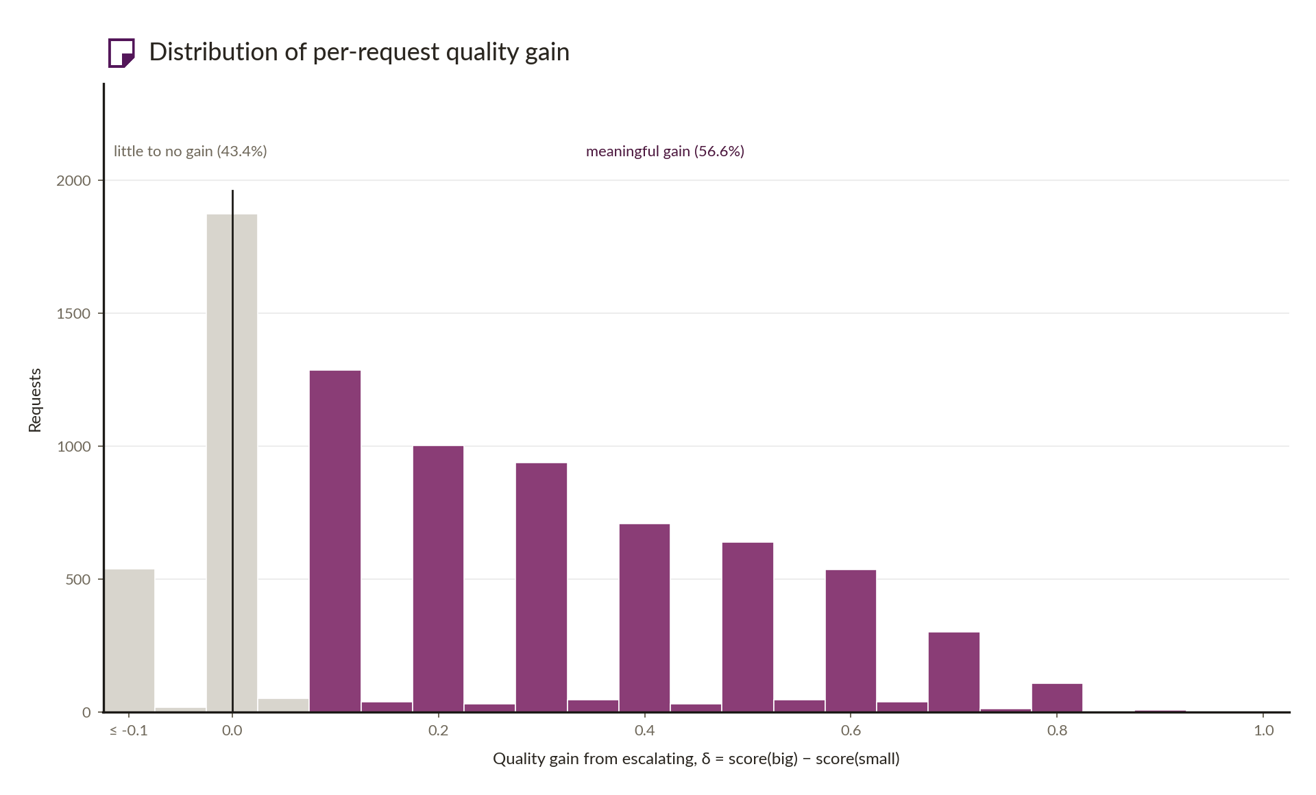
There are two regions, each with different economics:

• Requests with little to no gain (43.4%): the big model is indistinguishable from the small one, and on a small share it actually scores slightly worse, usually from grader preferences such as verbosity penalties.
• Requests with meaningful gain (56.6%): this is where essentially all of the value of routing lives.

The oracle frontier and router efficiency

Before fitting a predictor, it’s worth computing the policy that has access to the labels.

1. Label every request in the offline set with its true δᵢ and cᵢ
2. Sweep λ from high (escalate nobody) down to zero (escalate everybody), escalating request i whenever δᵢ − λcᵢ > 0
3. Record quality and added latency at each λ

That sweep traces the Lagrangian oracle frontier. This is the best a policy can do when it already knows the answers. This is also the same policy shape you could actually serve, which is what makes it the right thing to grade against.

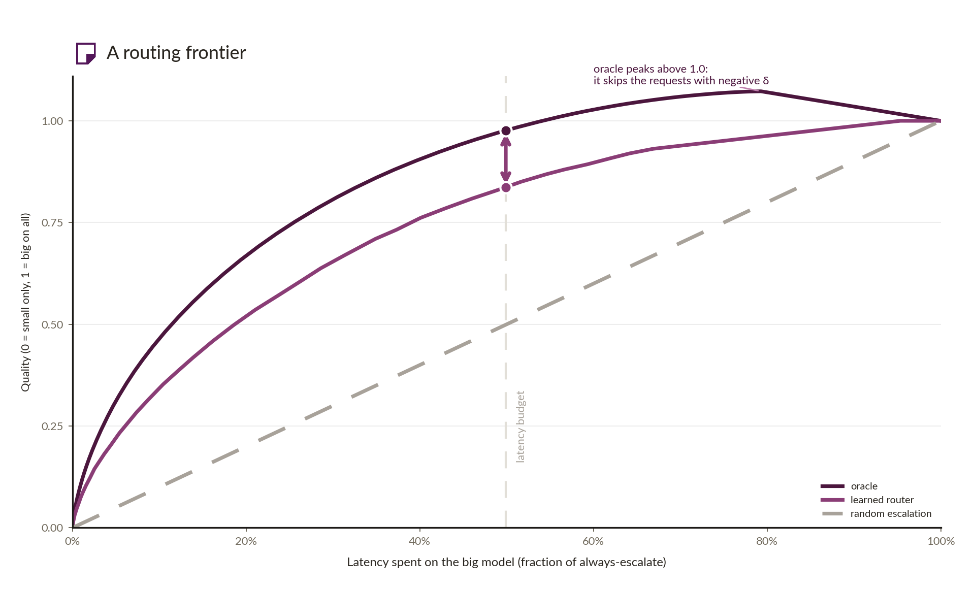
The oracle also tells you how much routing opportunity the benchmark contains at all. It is very similar to a Lorenz curve: the farther it bends away from the random diagonal, the more concentrated the model advantage is in a subset of requests.

Using the oracle also gives you a natural way to grade a router.

Router efficiency = (AUC_router − AUC_random) / (AUC_oracle − AUC_random)

In other words:

• the mean δ tells you how much gain exists
• the oracle tells you how routable that gain is
• the router-oracle gap tells you how much of the routing headroom remains

Router modeling

Feature engineering

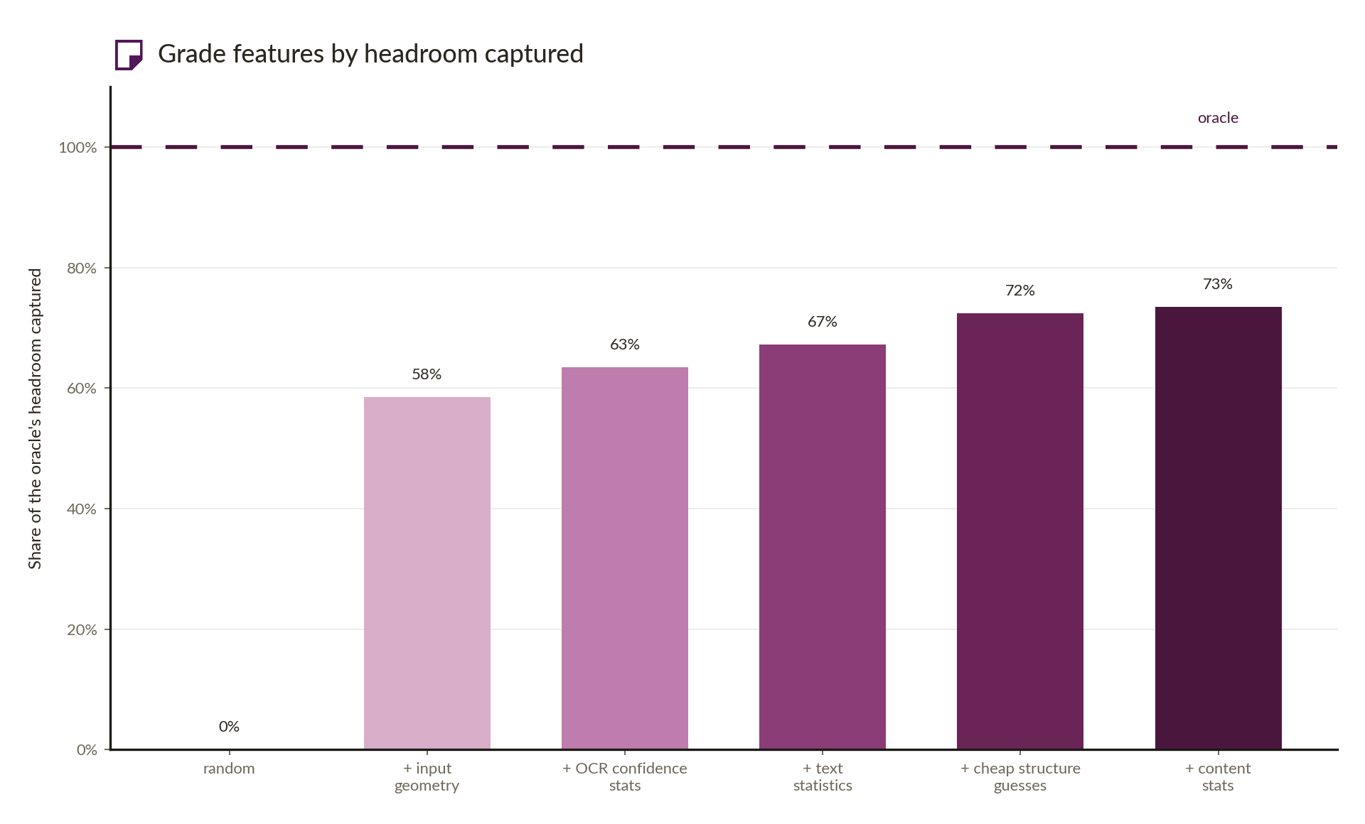
The router has to decide before the expensive model runs, so the feature set must be able to be computed at low latency: input size and shape, cheap content statistics, structural properties, and whatever metadata the API call already carries. All of it has to be fast, because featurization itself has a cost. Spending 50ms to decide whether to spend 900ms is reasonable, but spending 400ms means you’ve just added a third model candidate. For document parsing, some interesting features may be:

• Input geometry: page width, height, aspect ratio.
• OCR confidence stats: mean, min, 10th percentile, standard deviation.
• Text statistics: word count, line count, words per line, average word width, etc.
• Fast structure guesses: predicted row and column counts, whether merged spans are present, fraction of empty cells.
• Content stats: populated vs blank cells, header cells, numeric cells, character counts, etc.

Two predictions

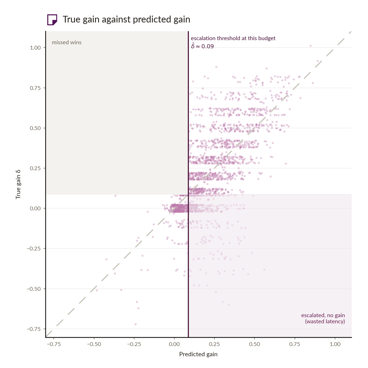
The serving rule is δ − λc > 0, so the natural thing to model is its two inputs: one predictor for δ̂, another for ĉ, combined at serving time as δ̂ − λĉ. Both are ordinary regressions over the same cheap feature vector, and neither needs to know anything about the eventual budget.

The models themselves can be simple and fast, for example, gradient-boosted trees over tabular features. In practice, ĉ is usually the easier prediction: added latency is dominated by quantities like input size that the router already observes. Most of the modeling work therefore goes into δ̂.

The main takeaway is model advantage

A router should learn where the big model is worth paying for. Difficulty is a property of the request, whereas δ is a property of the request and the model pair. Because δ̂ is fit to a specific pair of models, it needs to be refit when either model changes. λ, by contrast, can carry across model upgrades.

This routing experiment started with the same rigorous evals we use at Reducto to score model improvements and measure pairwise gains across our datasets, giving us a clear view of where additional model capability creates meaningful value. Model routing is a promising technique to use that signal to selectively apply more compute where it matters most.

Written by Apurv Gandhi and the Reducto ML team. Edited by Palak Agarwal.

Additionally, if these types of problems excite you, apply to join our team on our careers page.